Overview
Single constituent plots in Plan View can be produced in EnviroInsite with data from EQuIS. Data that can be plotted includes chemical analytical results, water quality parameters, and water elevations. There are several different types of two-dimensional (2D) single constituent plots in EnviroInsite, which are described in the table below.
Plot Type |
Plot Description |
|---|---|
Post Data |
Simple labels with observation or result values posted at monitoring locations. |
2D Contours |
Fill or line contours of interpolated constituent values over an area. The difference between two contour lines is defined as the contour interval, which indicates the relative slope of the surface. |
Classed Posts |
Color-coded symbols posted at monitoring locations that are based on grouping the data into discrete classes (bins). The color and radius of the symbol are dependent on the value of the selected constituent at that monitoring location. |
Exercise Scenario
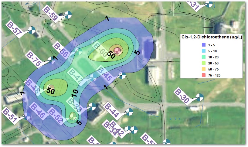
We want to evaluate the spatial distribution for a specific chemical of concern, Cis-1,2Dichloroethene, in groundwater. This will be accomplished by generating and adding post values and contour plots on our aerial map.
|
Use single constituent plots to understand the spatial distribution of chemicals of concern. |
|
Exercise Objectives |
•Generate Post Data
•Create Contours
Skills, Software and Permissions Required
•.NET Framework 4.6 or higher must be installed on the workstation
•EnviroInsite 2016 must be installed on the workstation
•Read/write permissions are required for the desired facilities
|
Objective: Generate Post Data |
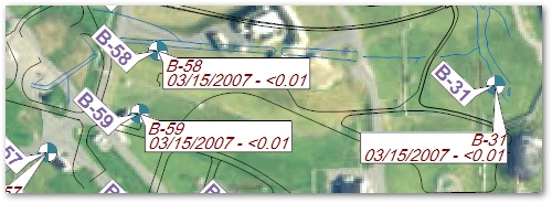
Generate post data at each location to add simple labels with concentration values and leaders.
1.If necessary, re-open the saved "insite1.vizx" file from the previous exercise.
2.Select Plot> 2D Data> Post.
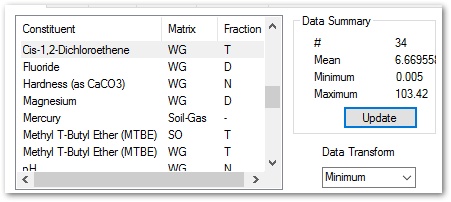
3.Select the desired constituent.
For this exercise, select Cis-1,2–Dichloroethene with a matrix of WG and a fraction of T.
4.Under Data Transform, select Maximum.
5.Click the Update button in the Data Summary box.
5.Select the Browse button from the bottom-left of the Post Observations dialog box to see the selected data in tabular view.
6.Scroll to the right to find the Value column.
7.Right-click on the Value header and select Sort Descending.
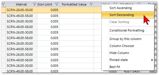
7.Select the Close button to return to the Post Observations dialog box.
8.The queried area, by default, is defined by the limits of the data. Select Draw Rectangle to change the extent of the area query limits.
9.Single-click to set the preferred top-left and bottom-right corner in the plan view.
10.Select the Options tab.
11.Check the Plot Labels and Show Date boxes.
12.Select the OK button.
13.Note the labels include the date on which the maximum result occurred at that location.
|
To open the Post Observations dialog box to edit an aspect of the post file, either double left-click on any post label or right-click on any post label and then select Edit. |
14.Select Edit> EQuIS Options.
15.Select the Default Units tab.
16.Verify the units selected by EnviroInsite for any given constituent are appropriate. If they are not, they may be changed on this tab.
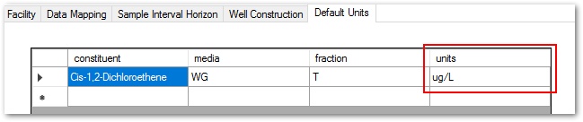
17.After making any necessary changes to the units, select the OK button.
|
Objective: Create Contours |
Contours are the interpolation of measured values onto a rectangular mesh. Inverse distance, kriging, and natural neighbor are the available interpolation methods.
|
Inaccurate data patterns may be portrayed and used to make decisions if sufficient consideration is not given to locations of non-detects, identification of plume extents, and many other criteria. It is important to understand both the function of the available tools in EnviroInsite AND the potential impact of the various options and interpolation methods. |
1.Un-check the Post Values layer from the Plot Control panel to turn the layer off.
2.Click Plot> 2D Data> Contour.
3.On the Query tab, select the desired constituent.
For this exercise, select Cis-1,2–Dichloroethene with Media of WG and Fraction of T.
4.Select the desired Data Transform, such as Maximum.
5.Under Data Summary select the Update button to refresh the statistics.
|
Click on the Browse button on the bottom left corner of the Post Observations dialog box to view the data that has been queried. |
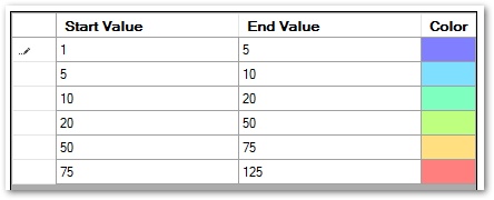
6.From the bottom of the Intervals tab, select Set Intervals.
7.Then select Set Default to establish the default contour levels.
8.Change these default contour values as desired by entering values into the End Value column.
For this exercise, change these default contour values to: 5, 10, 20, 50, 75, 125 by entering these values into the End Value column.
Change the Start Value of the first interval to 1.
9.Select the Format tab.
10.On the Format tab set the desired % Transparency, such as 50.
11.On the Interpolation tab select Kriging as the interpolation Method, and leave all the other parameters as defaults.
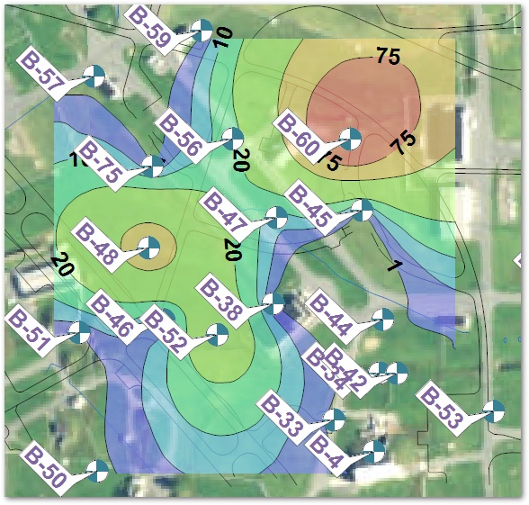
12.On the Grid tab, select Draw Grid to alter the extent of the contoured area.
13.Draw a box around the desired locations and then left-click when complete to return to the Grid tab of the Contour dialog box.
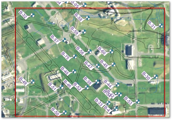
For this exercise, draw the box from B-57 to B-53, including all locations in-between.
|
The Grid defines the rectangular area over which the contours are generated. Modifying the grid confines the contour area to the portion of the facility where the contoured constituent is plotted. |
14.Click the OK button and EnviroInsite will create the contours in the selected area.
15.To make the well locations more visible, select the Contour layer in the Plot Control panel (on left of the screen) and drag it above the Wells layer.
Log-Transform Contours
Sometimes the data may be more appropriately contoured by using the logarithmic transform of the original data. This is common when there are localized hot-spots that are not necessarily representative of the concentration over a large area.
1.Right-click on the Contour icon in the Plot Control panel.
2.Select Duplicate.
|
Duplicating an object is a convenient way of creating a new plot feature with the same properties as the original and then making some small modification. |
3.Remove the check from the original contour.
4.Double-click on the newly created Contour plot in the Plot Control panel.
5.Select the Options tab.
6.Check Transform Data in the Log Transform box.
|
Further restrict the contour area by clicking on the Draw Polygon button of the Grid tab and drawing an irregular polygon around the area to be contoured. |
7.Select Grid.
8.Select Draw Polygon.
9.Single-click on the points on the map where the contour should be restricted.
10.Right-click to complete the polygon and return to the Contour options dialog box.
11.Click the OK button.